Compute transition frequency from custom clusters

This examples shows how to define two custom clusters of sensors and how to compute the corresponding theta-to-alpha transition frequency.

import mne
from transfreq import compute_transfreq_manual
from transfreq.viz import (plot_psds, plot_coefficients, plot_channels,
                           plot_clusters, plot_transfreq)
from transfreq.utils import read_sample_datapath
import os.path as op
import numpy as np
import matplotlib.pyplot as plt


# Define path to the data
subj = 'transfreq_sample'
data_folder = read_sample_datapath()
f_name = op.join(data_folder, '{}_resting.fif'.format(subj))

# Load resting state data
raw = mne.io.read_raw_fif(f_name)

# List of good channels
tmp_idx = mne.pick_types(raw.info, eeg=True, exclude='bads')
ch_names = [raw.ch_names[ch_idx] for ch_idx in tmp_idx]

# Compute power spectra
n_fft = 512*2
bandwidth = 1
fmin = 2
fmax = 30

sfreq = raw.info['sfreq']
n_per_seg = int(sfreq*2)

psds, freqs = mne.time_frequency.psd_multitaper(raw, fmin=fmin, fmax=fmax,
                                                bandwidth=bandwidth)

# Read channel positions
ch_locs = np.zeros((psds.shape[0], 3))
for ii in range(psds.shape[0]):
    ch_locs[ii, :] = raw.info['chs'][ii]['loc'][:3]

Out:

Opening raw data file /home/sara/Documenti/San_Martino_Alzhaimer/transition_frequency/transfreq/data/transfreq_sample_resting.fif...
/home/sara/Documenti/San_Martino_Alzhaimer/transition_frequency/examples/plot_manual_analysis.py:25: RuntimeWarning: This filename (/home/sara/Documenti/San_Martino_Alzhaimer/transition_frequency/transfreq/data/transfreq_sample_resting.fif) does not conform to MNE naming conventions. All raw files should end with raw.fif, raw_sss.fif, raw_tsss.fif, _meg.fif, _eeg.fif, _ieeg.fif, raw.fif.gz, raw_sss.fif.gz, raw_tsss.fif.gz, _meg.fif.gz, _eeg.fif.gz or _ieeg.fif.gz
  raw = mne.io.read_raw_fif(f_name)
    Range : 0 ... 29558 =      0.000 ...    59.116 secs
Ready.
    Using multitaper spectrum estimation with 57 DPSS windows

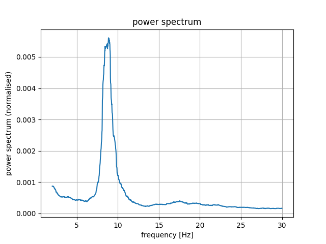
Plot power spectrum to visually chose theta and alpha ranges

plot_psds(psds, freqs, average=True)

Out:

<Figure size 640x480 with 1 Axes>

set theta and alpha ranges

alpha_range = [8, 9.5]
theta_range = [6.5, 7]

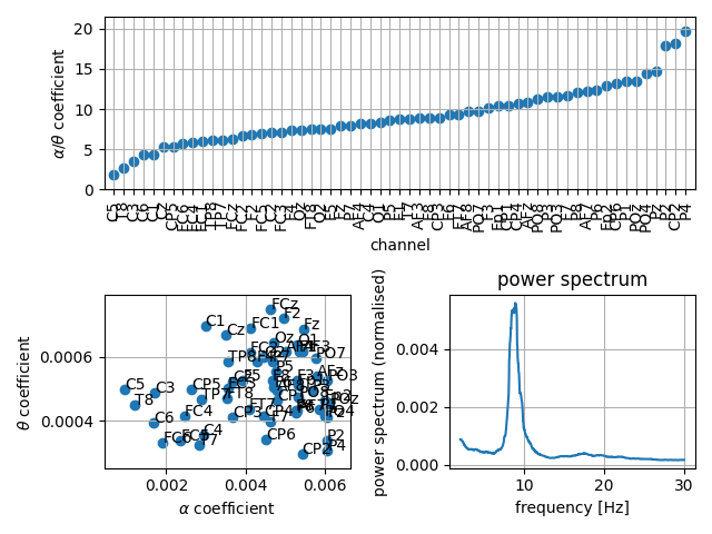
Plot alpha and theta coefficients. In the 1D visualisation the ratio between alpha and theta coefficients is plotted. In the 2d visualisation a scatter-plot of the alpha and theta coefficients is shown.

fig = plt.figure()
gs = fig.add_gridspec(2, 2)
ax1 = fig.add_subplot(gs[0, :])
plot_coefficients(psds, freqs, ch_names=ch_names, alpha_range=alpha_range,
                  theta_range=theta_range, mode='1d', ax=ax1, order='sorted')
ax2 = fig.add_subplot(gs[1, 0])
plot_coefficients(psds, freqs, ch_names=ch_names, alpha_range=alpha_range,
                  theta_range=theta_range, mode='2d', ax=ax2)
# Plot the corresponding averaged power spectra.
ax3 = fig.add_subplot(gs[1, 1])
plot_psds(psds, freqs, average=True, ax=ax3)
fig.tight_layout()

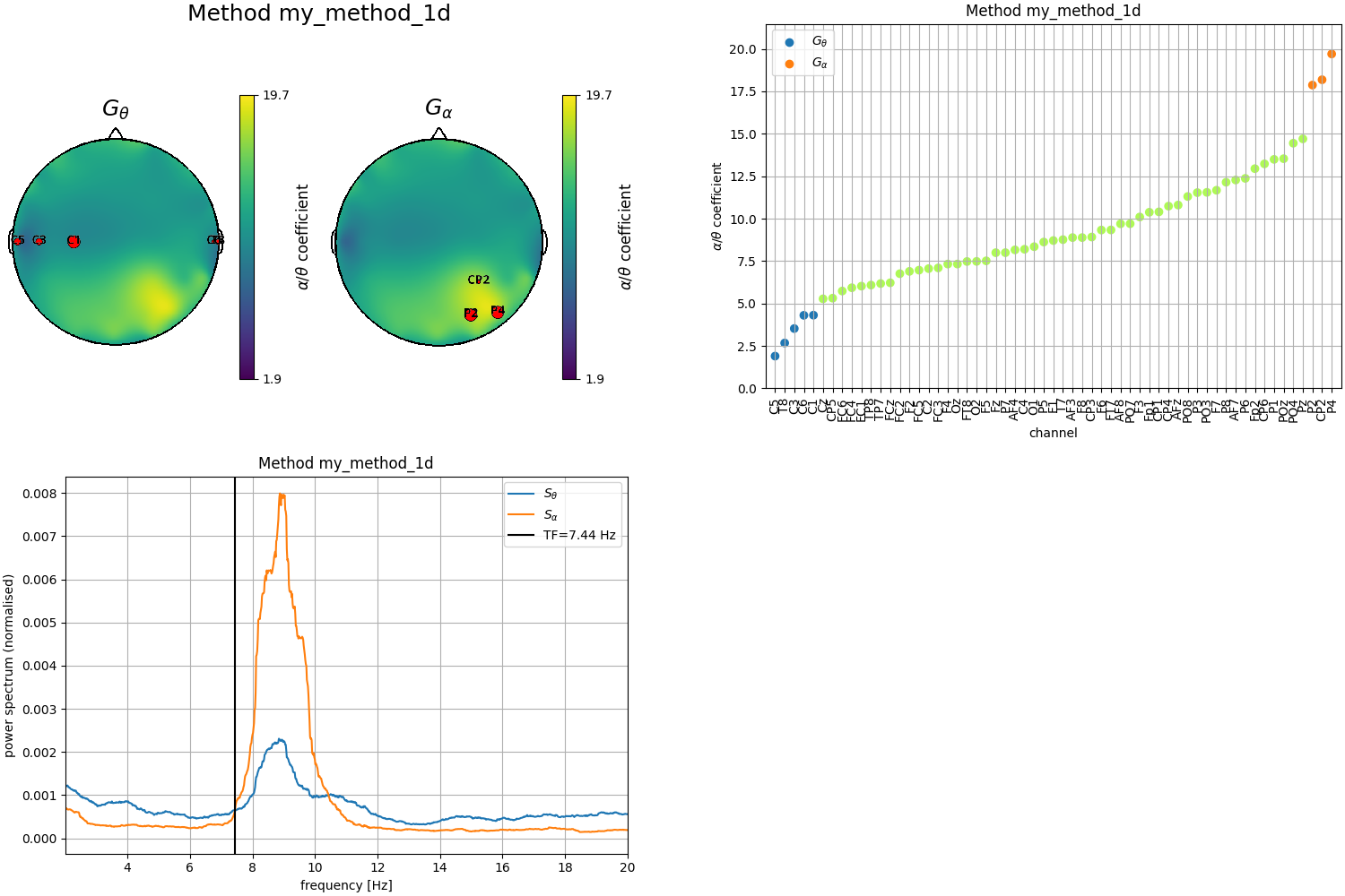
Chose channels from the figure to manually define the clusters and compute the corresponding transition frequency

# First definition by looking at the 1D plot
theta_chs_1d = ['C5', 'C3', 'T8', 'C1', 'C6']
alpha_chs_1d = ['P4', 'P2', 'CP2']

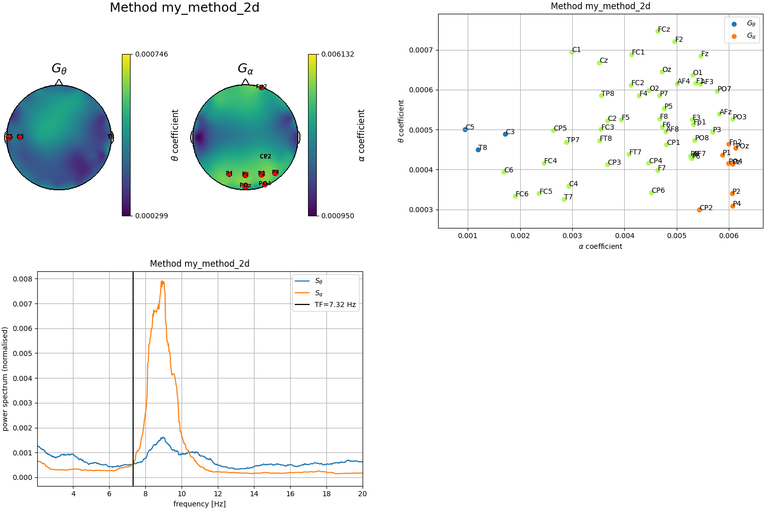
# Second definition by looking at the 2D plot
theta_chs_2d = ['C5', 'C3', 'T8']
alpha_chs_2d = ['P4', 'P2', 'Pz', 'CP2', 'POz', 'Fp2', 'PO4', 'P1']

tfbox_1d = compute_transfreq_manual(psds, freqs, theta_chs_1d, alpha_chs_1d,
                                    ch_names=ch_names, theta_range=theta_range,
                                    alpha_range=alpha_range, method='my_method_1d')
tfbox_2d = compute_transfreq_manual(psds, freqs, theta_chs_2d, alpha_chs_2d,
                                    ch_names=ch_names, theta_range=theta_range,
                                    alpha_range=alpha_range, method='my_method_2d')

Plot results obtained with the first definition of the clusters (1D)

fig = plt.figure(constrained_layout=True, figsize=(15, 10))
subfigs = fig.subfigures(2, 2, wspace=0.1)
plot_channels(tfbox_1d, ch_locs, mode='1d', subfig=subfigs[0,0])
ax1 = subfigs[0,1].subplots(1, 1)
plot_clusters(tfbox_1d, mode='1d', order='sorted', ax=ax1)
ax2 = subfigs[1,0].subplots(1, 1)
plot_transfreq(psds, freqs, tfbox_1d, ax=ax2)

Out:

<matplotlib.figure.SubFigure object at 0x7fafa498d310>

Plot results obtained with the second definition of the clusters (2D)

fig = plt.figure(constrained_layout=True, figsize=(15, 10))
subfigs = fig.subfigures(2, 2, wspace=0.07)
plot_channels(tfbox_2d, ch_locs, mode='2d', subfig=subfigs[0,0])
ax1 = subfigs[0,1].subplots(1, 1)
plot_clusters(tfbox_2d, mode='2d', order='sorted', ax=ax1)
ax2 = subfigs[1,0].subplots(1, 1)
plot_transfreq(psds, freqs, tfbox_2d, ax=ax2)

Out:

/home/sara/Documenti/San_Martino_Alzhaimer/transition_frequency/transfreq/viz.py:40: UserWarning: order can only be 'standard' if mode is '2d' or mode is None and method in tfbox is 3 or 4. Automatically switched to 'standard'
  "order can only be 'standard' if mode is '2d' or mode is None and method in tfbox is 3 or 4. Automatically switched to 'standard'")

<matplotlib.figure.SubFigure object at 0x7faf96f745d0>